Welcome to
Mathematics Laboratory
Mathematics Laboratory (ML for short) is a collection of tools for
communicating and getting to understand mathematical
concepts, relations, algorithms etc.
The idea is to make math easier to "get into" and understand by
visualization and interactivity, that can bring both
figures and formulas to life.
In our own courses, we have used ML as follows: matlab/ML is
used in class/lectures as an integrated tool for presenting
new material, and later the students use the same tools in computer
lab sessions and at home for further analysis and a full and
confirmed understanding of the new material.
Based on matlab
Physically, ML consists of a collection of matlab files (of .m
and .fig type), that you can easily download from this page and
then run from within the matlab program. That is, ML requires
matlab, and
you start the ML tools directly from the matlab >> prompt.
An example
For a first example, you may want to download the files
BISECT.fig and BISECTAdm.m,
the purpose of which is to present the Bisection algorithm for solving
equations of the form f(x) = 0.
To open this demonstration/lab tool, type open 'BISECT.fig' at
the matlab prompt. A new window should pop up, with the graph
y = f(x) of a sample function f(x), and a number of
buttons and text fields as follows:
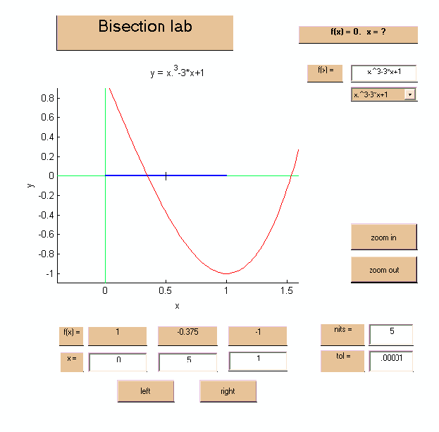
The idea is now for the user to select the subinterval hosting the zero of
the given function, by pressing one of the buttons left of right,
and then to repeat.
The idea is to give the students a more or less instant understanding
of the algorithm this way, through a demonstration in a lecture.
Further, as the remaining interval, after a number of steps, gets too small to
see easily, one is naturally led to rather use the corresponding
f(x)-values as a basis for which sub-interval to choose, and then
seek to write down the algorithm in terms of a logical "flow chart".
Based on the visualization of the Bisection algorithm offered by this "lab"
one may also discuss
- when to stop the bisection iterations?
- what is the answer/root delivered by the algorithm? (an interval or a particular x
in such an interval, which x is best?, ...)
- what is the remaining error?
- are there different error concept? (x-error vs.
f(x)/residual error ...)
- how are these related, which one should be used, how estimate the
x-error, ...
- is this the only solutions? ("uniqueness" considerations, zoom out..)
- existence considerations (for a general f(x))
- existence of "perfect" or "exact" solution
- ...
Implementation
We present the Bisection algorithm very early to our students, not so much because
of its qualities as a solver, but rather because of its conceptual simplicity,
and because implementing this method, which the students are set to do, involves
most of the basic programming "elements" (an iteration loop, conditional
statements, interesting logical considerations etc). That is, in our courses
the students first meet this method in class, then get the chance to experiment
on their own using the same tool in a lab session, and then to make their own
implementation of the method from a code shell. For an example of how
we have used these tools in a first math course for engineering students, see
www.math.chalmers.se/cm/education/courses/0304/intro/.
Other solvers
Similar tools exist in the form of a
FixedPointLab
for the fixed point iteration algorithm, for equations of the type
x = g(x),
and a NewtonLab for Newtons method.
As an introduction to general equation solvers of this form, just to present
the very idea of an iterative solution process, we have sometimes used
the ZoomSolveLab where the equation
f(x) = 0 is solved simply by
succesive graphing and zooming. The limitation of this method,
of course, is the difficulty to visualize the graph y = f(x) in higher
dimension, that is, to generalize to systems of equations.
Shipping
The latter "labs" have been "packed" into an archive and then "zipped" for easy
shipping in just one package. However, this means that you have to "unzip" and
"extract" the individual files at arrival.
Help
The FixedPoint and Newton labs above (and several others to be presented below),
come with a html help file that you start from within the
lab to get tips on how the lab may be used and suggested problems.
All labs are opened from the matlab prompt with the command
open 'labname.fig',
where labname is the name of the .fig file delivered with the package/lab
in question.
Polynomial approximation
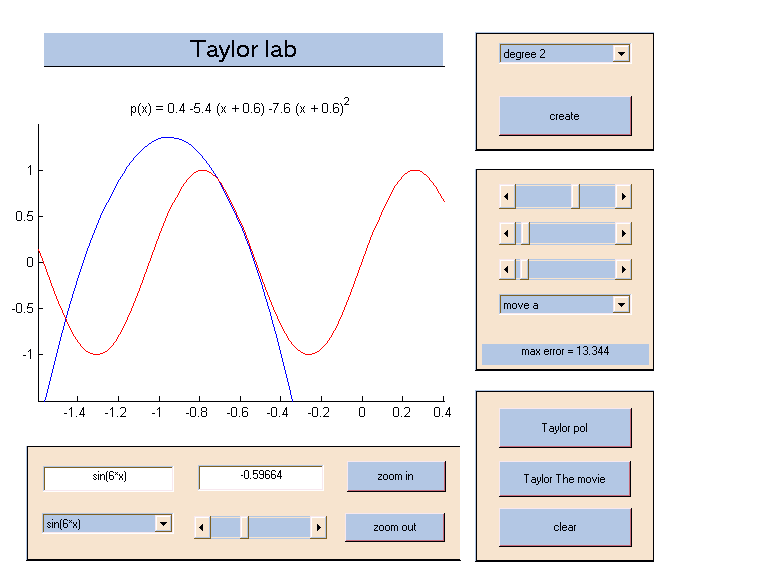
To help the students understand polynomial approximation, we
have developed a TaylorLab, for visualization
of Taylor polynomials,
and a PiecewisePolynomialLab for
undestanding approximation by
piecewise polynomial functions, used in modern computational methods
for solving differential euqations.
Differential equations
Differential equations come in many different forms. A lab tool for better
understanding so called two-point boundary value problems for second
order such equations can be found in
TwoPointBoundaryValueProblemsLab,
and a tool that presents the finite element method in this context can
be found in
TPBVPFEMLab.
These labs could be used as an
introduction
to computational mathematical modelling based on differential equations
and the finite element method using piecewise polynomial approximation.
Multidimensional calculus and Finite element methods
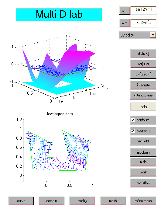
To support important parts of a multi-dimensional calculus course, we have developed
MultiDCalculusLab. In this you can learn about
visualization of multidimensional
fields using contour plots, vector plots, and graphs, get familiar with the basic
differential operators grad, div, rot and div
grad, and study the important integral theorems of Gauss, relating
divergence to boundary outflow, and Stokes, relating interior rotation to
a boundary work integral.
Once familiar with basic differential equation modelling in several dimensions, it
is natural to get introduced to the finite element method in its simplest
(multi-dimensional) form using the
FiniteElementLab,
and then the application
labs
PoissionsLab
(for Poisson or Heat type equations) and
NaviersLab
(for Naviers equations in elasticity).
Applications
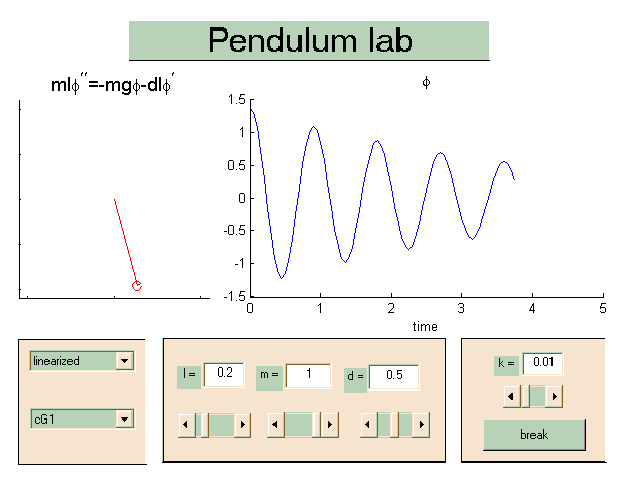
A few tools related to dynamical systems type applications can be
found in PendulumLab, specifically illustrating
the role of linearization,
in the context of the pendulum equation, but also the role of the discretization
method, where an important limitations of the classical explicit Euler method is
demonstrated (adds artificial numerical energy) with the conservative cG1
or trapezoidal method as a contrast.
Another tool demonstrates how more complicated mechanical systems can be modelled
and simulated using the same compuational technique in
MiniMechLab.
A third example involving dynamical systems is the
RoboticsLab.
In this lab
you can build a robot model, "joystick" the robot, and study also the inverse
kinematics problem by specifying a target point for the robot to move to.
New tools for studying the simplest first and second order dynamical systems (ode's)
is under development.
Algebra and geometry
On a more basic level, the
VectorCalculatorLab lab, may be used
to illustrate
elementary vector algebra, matrix-vector multplication, orthogonal projection,
the algebra for complex numbers etc, etc.
Similarly,
EuclidLab
is supposed to illustrate how a system of linear
equations may be interpreted geometrically two ways, in the x-space or in
the column-space, and also the concept of a over-determined such
system and the least square approximate solution.
The Graph Gallery
The
GraphGallery
is thought of as a gallery with a "first floor" for graphs
of simple one-variable functions, with rooms "exibiting" graphs of various types of
such functions, like polynomials, exponentials, trigonometic functions etc, and a
"second floor", with functions of several variables and vector valued functions.
A separate tool has been designed for mappings in terms of complex variables and can
be found in ComplexLab.
Basics math
We have also developed tools for very basic math concepts such as
SequencesLab,
LipschitzLab,
InverseFunctionLab,
LinearizationLab,
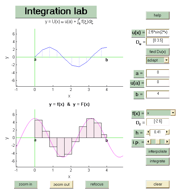
IntegrationLab.
Math Road map
Most of the demonstration and lab tools mentioned above can be accessed through a
Road Map tools called MathRoadMap. What this interface does is simply to
open a specific tool among the ones mentioned above.
Development
Many of the tools presented here are still under development, may not always
function as desired. Please feel welcome to interact and participate in the further
development by presenting constructive feedback whenever deeped appropriate. You are
also welcome to suggest new tools covering new areas of math. For example, a tool
illustrating partial derivatives and optimization is under construction, and another
one illustrating forurier analysis is also to be added.
Platform independence
Most of the existing labs were developed on a unix platform while some may have been
modified for a better look on a pc system. If you find some of these labs not so
"good looking", you may interprete this as the lab being designed for another environment.
Hopefully, a "next version" of these labs will be able to adapt to the platform on
which they are run.
Example code and Code shells
To support our courses we have also produced a large number of .m files
with example code for various purposes, and code shells which could consist
of just a "header" for code specifying what the code (when written) should do, to code
with some (key) parts missing for students to fix. Below you find a list of some of this
code with a short specification of its purpose.
Disclaimer
ML comes with no guarantee to give correct solutions. In fact, there are known bugs
and you can expect to find lots of "new" bugs in many of these lab tools. Occationally
you may even find that matlab will "crash" as a result of trying to run some of these
labs.